2. Using EDRep

We focus on the main function of this package, CreateEmbedding, which is the implementation of Algorithm 1 of our paper. The function is called in the following way

res = CreateEmbedding(Pv)

Here Pv is a list of scipy sparse arrays. The EDRep algorithm generates an embedding from a probability matrix P. In this case, we should write Pv = [P]. The sparsity of P is crucial to keep high efficiency. Suppose that P can be written as the product of sparse matrices (\(P = P_3P_2P_1\)). Even if all the matrices in the product are sparse, P can be dense. In our implementation, we explicitly consider this factorization as a possible input and would have Pv = [P1, P2, P3]. This allows a much faster implementation. We now show this on some synthetic data.

Remark: note that the matrices are ordered in the opposite direction.

# load the needed package
import numpy as np
from scipy.sparse import csr_matrix
from time import time
import matplotlib.pyplot as plt
import pandas as pd
from scipy.sparse import diags

from EDRep import CreateEmbedding

2.1. The main input and output of the function

# generate a sequence Pv to be embedded. Each matrix should be a probability matrix
n = 2500
At = [np.random.binomial(10, 5/n, (n, n)) for _ in range(5)]
Pv = []

for A in At:
    v = np.maximum(1, A@np.ones(n))
    Pv.append(csr_matrix(np.diag(v**(-1))@A))

# we compare the execution time of the two versions of the algorithm 
t0 = time()
np.random.seed(123)
P = np.prod(Pv[::-1])
res_agg = CreateEmbedding([P])
print(f'Execution time aggregated version: {time() - t0}\n')

t0 = time()
np.random.seed(123)
res = CreateEmbedding(Pv)
print(f'Execution time efficient implementation: {time() - t0}')

## PLOT
plt.scatter(res.X.flatten(), res_agg.X.flatten(), alpha = 0.1, color = 'dodgerblue')
plt.xlabel('Multiplication from left to right', fontsize = 16)
plt.ylabel('Multiplication from right to left', fontsize = 16)
plt.show();

Running the optimization for k = 1
Execution time aggregated version: 20.11892533302307

Running the optimization for k = 1
Execution time efficient implementation: 2.27961802482605

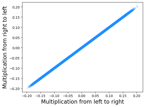
To access the embedding we simply need to type res.X. Let us check that the embeddings obtained by the two implementations are actually the same.

Remark

We simply created random entries to test the algorithm. This implies that the matrix \(P\) can be non-symmetric and weighted. The only >requirement we ask is that it is non-negative and the its rows sum up to \(1\).

2.2. Other inputs

All other inputs of this function are optional. We describe them here for convenience.

• dim: this is the size of the embedding dimension and it should be an integer.

• n_epochs: this is the number of gradient descent steps from the initial condition and it should be an integer.

• eta: this is the initial value of the learning parameter

• verbose: if True it prints the progress bar and otherwise it doesn’t.

• k: this sets the order of the multivariate Gaussian approximation presented in the paper. If this parameter is not specified it is set to \(1\) by deault. If it is set to \(k > 1\), the algorithm is run for \(k = 1\), then a label partition is inferred on \(k > 1\) clusters and it is rerun for the updated parameters.

Let us now focus on other three optional inputs that are less straightforward.

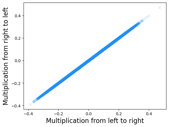
2.2.1. sum_partials

This variable is a Boolean. If it is set to True it assumes that \(P \propto P_1 + P_2P_1 + P_3P_2P_1\). We thought of this to easily model random walks of varying length on graphs. Let us check!

P = [Pv[0]]
for t in range(1, len(Pv)):
    P.append(Pv[t]@P[-1])
P = np.sum(P)/len(Pv)

t0 = time()
np.random.seed(123)
res_agg = CreateEmbedding([P], sum_partials = False)
print(f'Execution time aggregated version: {time() - t0}')

t0 = time()
np.random.seed(123)
res = CreateEmbedding(Pv, sum_partials = True)
print(f'Execution time efficient implmentation: {time() - t0}')

## PLOT
plt.scatter(res.X.flatten(), res_agg.X.flatten(), alpha = 0.1, color = 'dodgerblue')
plt.xlabel('Multiplication from left to right', fontsize = 16)
plt.ylabel('Multiplication from right to left', fontsize = 16)
plt.show();

Running the optimization for k = 1
Execution time aggregated version: 19.37092089653015
Running the optimization for k = 1
Execution time efficient implmentation: 2.8942296504974365

2.2.2. sym

This is a boolean variable that allows one to use the asymmetric version of the algorithm. If sym = False, instead of optimizing over \({\rm SoftMax}(XX^T)\), two embedding matrices are used, and the loss function features the term \({\rm SoftMax}(XY^T)\), with \(X \in \mathbb{R}^{n \times d}\) and \(Y\in\mathbb{R}^{m \times d}\) with \(m\) potentially different from \(n\). In other words, this allows the user to embed a rectangular matrix \(P\in\mathbb{R}^{n \times m}\) in which the rows and the columns span different spaces.

We provide a simple use case from matrix completion systems. We consider the RetailRocket dataset (Zykov et al., 2022) which contains a sequence of events collected from a commerce website. Each event is associated with a time stamp, a user id, an item id, and an event type that can be “view”, “add to cart”, or “transaction”. We create a matrix \(A_{ia}\) by letting its entry be equal to \(1\) if user \(i\) interacted at any time with item \(a\), and we let \(P\) be the row-normalized version of \(A\). We then suppose we only observe a fraction of the events and use embedding vectors to guess whether a non-observed edge exists or not. We train the embedding with the non-symmetric version of the EDRep algorithm and then we create two samples of edges: one from the test set, the other composed of random node pairs. We then compute the F1 score, assuming that if \(x_i^Ty_a > 0\), then the edge exists.

# load the dataset
df = pd.read_csv('data/events.csv')

# preprocess the data

# create an edge list between visitors and items
df = df.groupby(['visitorid', 'itemid']).sum().reset_index()[['visitorid', 'itemid']]

# map visitor ids to integers
all_visitor_id = df.visitorid.unique()
n = len(all_visitor_id)
visitor_mapper = dict(zip(all_visitor_id, np.arange(n)))

# map item ids to integers
all_item_id = df.itemid.unique()
m = len(all_item_id)
item_mapper = dict(zip(all_item_id, np.arange(m)))

df.visitorid = df.visitorid.map(lambda x: visitor_mapper[x])
df.itemid = df.itemid.map(lambda x: item_mapper[x])

print('Pre-processed data:\n')
df

Pre-processed data:

	visitorid	itemid
0	0	0
1	0	1
2	0	2
3	1	3
4	2	4
...	...	...
2145174	1407575	92255
2145175	1407576	36504
2145176	1407577	61448
2145177	1407578	22299
2145178	1407579	22895

2145179 rows × 2 columns

# probability of observing an edge
p = 0.7
nrows = len(df)
dim = 8

# create train and test sets
train_bool = np.random.binomial(1, p, nrows) == 1
df_train = df[train_bool]
df_test = df[~train_bool]

# obtain the probability matrix from the train set
A = csr_matrix((np.ones(len(df_train)), (df_train.visitorid, df_train.itemid)), shape = (n,m))
d = np.maximum(1, A@np.ones(m))
D_1 = diags(d**(-1))
P = D_1@A

# compute the embeddings
res = CreateEmbedding([P], dim = dim, sym = False)

Running the optimization for k = 1
[========================>] 100%

tp = np.mean(np.sum(res.X[df_test.visitorid] * res.Y[df_test.itemid], axis = 1) > 0) 
fp = 1 - tp

idx1, idx2 = np.random.choice(np.arange(n), len(df_test)), np.random.choice(np.arange(m), len(df_test)) 
tn = np.mean(np.sum(res.X[idx1] * res.Y[idx2], axis = 1) < 0)
fn = 1 - tn

F1 = 2*tp/(2*tp + fp + fn)
print(f'F1 score: {F1}')

F1 score: 0.7113445864413995