1. Estimation of the SoftMax normalization constant

Here we show how to use the computeZest function of the EDRep package that computes the normalization constants

\[ Z_i = \sum_{i = 1}^n e^{x_i^Tx_j} \]

The function is called as

res = computeZest(X, indices, k)

where, X is an array containing in its rows the vectors \(x_i\). indices is the set of indeces \(i\) for which \(Z_i\) has to be returned.

REMARK: our estimation method can compute \(Z_i\) for all indeces in parallel. In this case, one needs to set indices = np.arange(n), where n is the number of rows of X.

The function features an additional parameter k which is optional and it is the order of the mixture model. The larger k, the higher the accuracy, but the longer the computational time. The output of this function is a class whose elements are described as follows:

• res.Zest (array): array containing the Z_i values corresponding to the indices

• res.ℓ (array): label vector

• res.μ (array of size (d x k)): it contains the mean embedding vectors for each class

• res.Ω (list of k arrays of size (d x d)): it contains the covariance embedding matrix for each class

• res.π (array of size k): size of each class

1.1. Load the relevant packages

# load useful packages for data processing and plotting
import numpy as np
import matplotlib.pyplot as plt
import pandas as pd
import csv

# load the computeZest function from the EDRep package
from EDRep import computeZest

# in this script we implemented a competing method as a reference
from src.EstimateZ import *

1.2. Load an embedding matrix

In the data folder, add a file called 0.txt, taken from https://vectors.nlpl.eu/repository/ (the file with ID 0). We use this file to show how to use our function. Note that we perform the operation X = X/np.mean(norms) because our result holds for embedding vectors with bounded norms.

# load the data
X = pd.read_csv('data/0.txt', skiprows = 1, on_bad_lines='skip', sep = ' ', header = None, quoting=csv.QUOTE_NONE,
                encoding='latin-1')
X.set_index(0, inplace = True)
X = X.dropna(axis = 1)
X = X.values

# number of indeces and embedding dimensions
n, dim = np.shape(X)

# rescale the norms of the embedding vectors
norms = np.sqrt(X**2@np.ones(dim))
X = X/np.mean(norms)

1.3. Compute the normalization constants

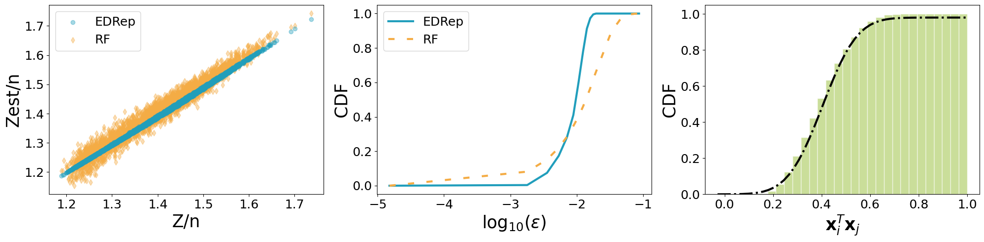
We compute the normalization constants for \(N\) indices (and not for the full dataset) because we compare them with the exact computation which is very time-consuming. We compare our calculation with a method based on Random projections that exploits the kernel method.

# select some random indices
N = 3000
indices = np.random.choice(n, N, replace = False)

# exact computation
Z = np.sum(np.exp(X[indices]@X.T), axis = 1)

# EDRep
res = computeZest(X, indices, k = 1)

# RF
D = 1000
Z_RFM = RFM(X, D, indices)

fig, ax = plt.subplots(1, 3, figsize = (20, 5))

colors = ['#219ebc', '#F4AC45']

ls = ['-', (0, (3, 6)), (0, (1,1))]
labels = ['EDRep', 'RF']

# scatter plot of exact vs estimated Z
ax[0].scatter(Z/n, res.Zest/n, color = colors[0], alpha = 0.4, marker = 'o', zorder = 1, label = 'EDRep')
ax[0].scatter(Z/n, Z_RFM/n, alpha = 0.4, color = colors[1], marker = 'd', zorder = 0, label = 'RF')
ax[0].legend(fontsize = 18)
ax[0].set_xlabel('Z/n', fontsize = 25)
ax[0].set_ylabel('Zest/n', fontsize = 25)
ax[0].tick_params(axis='both', which='major', labelsize=18)

# CDF of the error
eps = [np.abs(Z - res.Zest)/n, np.abs(Z - Z_RFM)/n]
emin, emax = np.min(np.concatenate(eps)), np.max(np.concatenate(eps))
tv = np.linspace(np.max([-5, emin]), emax)

for i in range(len(eps)):
    ax[1].plot(np.log10(tv), [np.mean(eps[i] < t) for t in tv], color = colors[i], linewidth = 3, linestyle = ls[i], label = labels[i])
    
ax[1].set_xlabel(r'${\rm log}_{10}(\epsilon)$', fontsize = 25)
ax[1].set_ylabel('CDF', fontsize = 25)
ax[1].tick_params(axis='both', which='major', labelsize=18)
ax[1].legend(fontsize = 18)


# fit of the scalar product distribution

# select a random index
α = np.random.randint(n)
    
ax[2].hist(X[α]@X.T, bins = 30, edgecolor = 'white', color = '#a7c957', alpha = 0.6,
                    density = True, label = 'Empirical', cumulative = True)

m = np.mean(X[α]@X.T) 
s = np.sqrt(np.var(X[α]@X.T))

t = np.linspace(1.03*np.min(X[α]@X.T), np.max(X[α]@X.T))
π, μ, σ2 = res.π, res.μ, res.Ω

y = np.sum(np.diag(π/n)@np.array([Normal(X[α]@μ[b].T, X[α]@σ2[b]@X[α], t) for b in range(len(μ))]), axis = 0)
ax[2].plot(t, np.cumsum(y)*(max(t)-min(t))/len(t), color = 'k', linewidth = 3, linestyle = '-.', label = 'mvGaussian')
ax[2].tick_params(axis='both', which='major', labelsize = 18)
ax[2].set_xlabel(r'$\mathbf{x}_i^T\mathbf{x}_j$', fontsize = 25)
ax[2].set_ylabel('CDF', fontsize = 25)


plt.tight_layout()
plt.show();